View a video from Hyungkyung Kim explaining how to navigate the Genetic Loci Clustering interfaces:
Research methods
I) Pipeline for input matrix for clustering
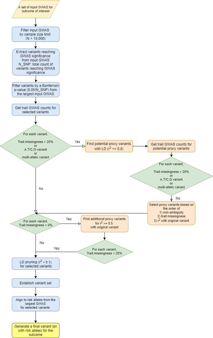
An overview of preprocessing steps for variants and traits used for generating the input matrix for variant-trait association clustering analysis is illustrated in Figures 1 and 2.
Variant selection
To obtain a comprehensive set of independent genetic variants associated with type 2 diabetes (T2D), coronary artery disease (CAD) and chronic kidney disease (CKD), we gathered GWAS summary statistic datasets deposited in the AMP-CMD Knowledge Portal. We required the GWAS to have sample sizes larger than 10,000 in order to reduce the likelihood of false positive results and focused on studies with populations of predominantly European ancestry in order to minimize heterogeneity across studies. Thirteen GWAS datasets including DIAMANTE and DIAGRAM (DIAbetes Genetics Replication And Meta-analysis) were included as input studies for T2D genetic loci, 6 datasets including CARDIoGRAM for CAD, and 39 datasets for CKD. Since there are not many known CKD variants, we added other relevant outcome GWAS such as diabetic kidney disease (DKD), end-stage renal disease (ESRD), eGFR and cystatin C to be inclusive.
From the selected GWAS datasets for each outcome, we first extracted variants reaching genome-wide significance (P < 5×10⁻⁸) and then ensured variant signals replicated in the largest GWAS study with a Bonferroni p-value (0.05/N, N: number of variants before filtering). For variants that were multi-allelic, ambiguous (A/T or C/G), or represented in less than 80% of trait GWAS datasets, we found proxy variants in linkage disequilibrium (LD) with the initial variants using HaploReg v4.1 that were non-ambiguous (no A/T or C/G) and were present in at least 80% of trait GWAS. One proxy variant was selected to represent each locus based on (in order) 1) non-ambiguity, 2) trait GWAS representation and 3) high LD (r2 >= 0.8) with the initial variant. Ambiguous variants were avoided due to potential error of using the incorrect allele in extracting data from summary statistic files.
This set of variants filtered through the process described above to optimize their use in generating a variant-trait matrix were then LD-pruned using the LDlinkR package in R by LD Link. We performed aggressive LD-pruning to remove variants with r2 >= 0.1 with an index variant. When performing the LD-pruning, a variant with lower p-value for the outcome was prioritized to be retained. We then identified the risk alleles for the outcome of interest with OR > 1 in the largest available GWAS containing that variant and aligned all variants using their risk increasing alleles.
For combined analysis of T2D, CAD and CKD, we first combined variant lists for all three outcomes, LD-pruned the variants if two variants from different outcomes were in LD (r2 >= 0.5) and selected the one with lower p-value with a label of the other outcome added (e.g. ABO_T2D_CAD). If the risk alleles for the two outcomes were different, an additional “_neg” label was added for the other outcome (e.g. FGF5_CKD_CADneg). The remaining set of variants and the union of selected traits for three outcomes were used for clustering analysis.
Figure 1. Overview of variant preprocessing pipeline
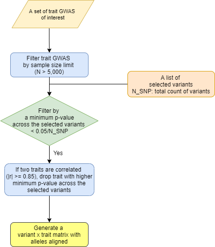
Trait selection
For trait selection, we utilized summary statistics available for GWAS of glycemic traits, anthropometric traits, vital signs, and additional laboratory measures in the CMD Knowledge Portal. We restricted to GWAS with sample sizes larger than 5,000 to reduce false positive associations and selected studies from predominantly European populations to maximize homogeneity, as noted above. Additionally, we included serum biomarker GWAS results available from the UK Biobank. Our goal was let the genetics guide which traits were included in the clustering analysis, and thus traits were used only if the minimum P value across the final set of variants was less than a Bonferroni P value cutoff of 0.05/N_final_variants; thus all the traits included in the clustering analysis had robust associations with at least one variant. If two traits were highly correlated (|r|>= 0.85), the trait with higher minimum p-value across all variants was removed.
For the selected lists of variants and traits, we generated a matrix of standardized effect sizes for variant-trait associations from GWAS by dividing the estimated regression coefficient beta by the standard error using the GWAS summary statistics. To account for the differences in sample size across studies for phenotypes, we scaled the standardized effect sizes in a two-step process: each value was divided by the square root of the sample size for each variant in each trait GWAS, then all elements were multiplied by the mean of square root of median sample size across all SNPs.
Figure 2. Trait preprocessing pipeline
II) Bayesian non-negative matrix factorization (bNMF) clustering
We generated standardized effect sizes for variant trait associations from GWAS by dividing the estimated regression coefficient beta by the standard error, using the GWAS summary statistic results. To address the marked differences in sample size across studies and allow for a more uniform comparison of phenotypes across studies, we scaled the standardized effect sizes by the square root of the study size, as estimated by mean sample size across all SNPs, forming the variant-trait association matrix Z.
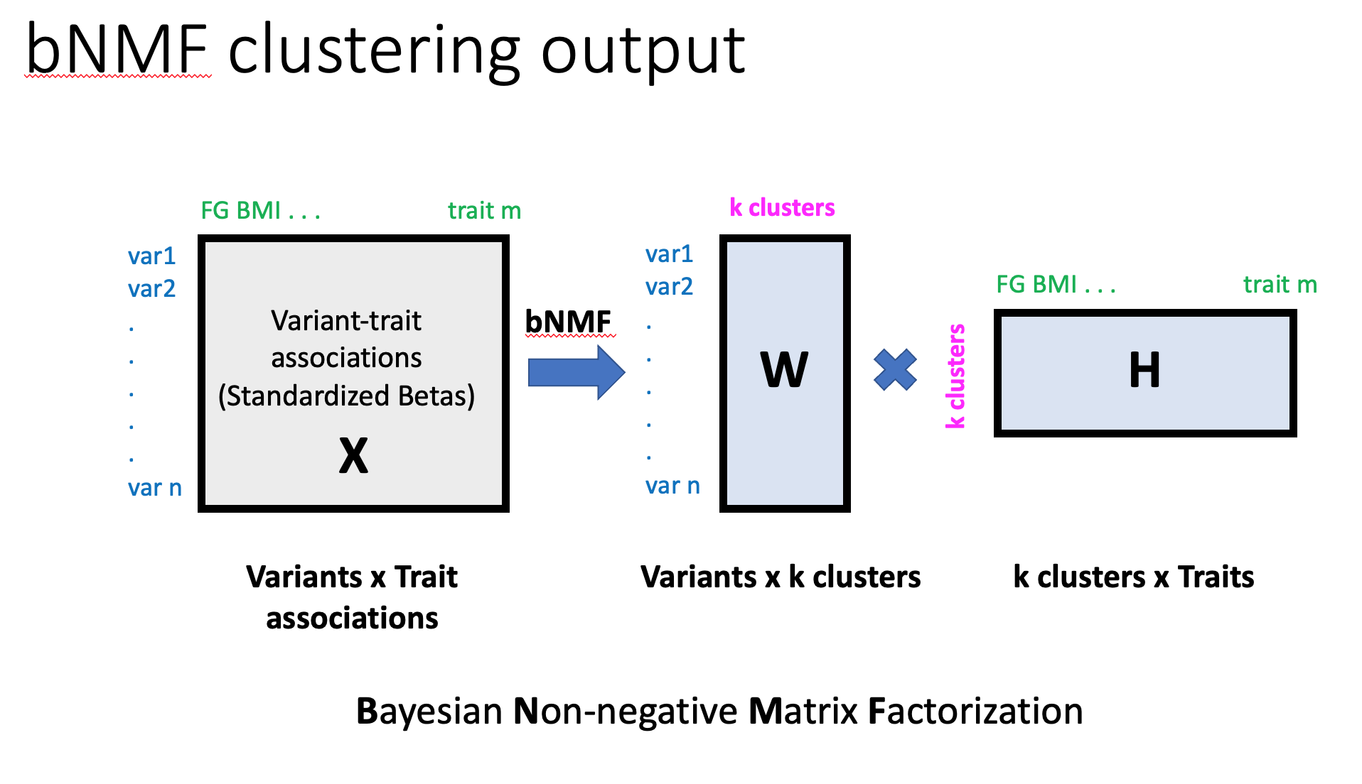
To enable an inference for latent overlapping modules or clusters embedded in variant-trait associations, we modified the existing bNMF algorithm to explicitly account for both positive and negative associations. Each column of Z split into two separate entities: one contained all positive z-scores, the other all negative z-scores multiplied by −1, and setting zero otherwise, leading to the association matrix X comprised of doubled traits with positive and negative associations to variants.
Then, bNMF factorizes X into two matrices, W and HT, with an optimal rank K, as X ~ WH, corresponding to the association matrix of variants and traits to the determined clusters, respectively (see Figure 3). Determining the proper model order K is a key aspect in balancing data fidelity and complexity. bNMF is designed to suggest an optimal K best explaining X at the balance between an error measure, ||X−WH||2, and a penalty for model complexity derived from a nonnegative half-normal prior for W and H. The defining features of each cluster are determined by the most highly associated traits, which is a natural output of the bNMF approach. The results of clustering provide cluster-specific weights for each variant (W) and trait (H).
Figure 3. bNMF clustering output
Reference:
High-throughput genetic clustering of type 2 diabetes loci reveals heterogeneous mechanistic pathways of metabolic disease.
Kim H, et al.
Diabetologia. 2023 Mar;66(3):495-507. doi: 10.1007/s00125-022-05848-6.
PMID: 36538063